Dimension reduction

class: center, middle, inverse, title-slide

.title[
# Dimension reduction
]
.subtitle[
## Using PCA, t-SNE and MDS to explore high-dimensional omics data
]
.author[
### Laurent Gatto (UCLouvain, BE)
]
.date[
### CSAMA – 26 May 2026
]

---

class:

### What is DR?

- **Dimentionality reduction** (also called ordination) is part of
  unsupervised machine learning.
- Map high-dimensional (HD) data in a low-dimensional space (LD)
  (latent space, embedding) while **preserving structure**
  (i.e. signal, could be biological and/or technical) as *much as
  possible*.

???

The *as much as possible* is of course central here!
--

#### Applications

- Used for data **exploration** and data **communication**.
- Use cases: visualisation and feature selection/transformation.

.left-col-50[

]

.right-col-50[

<img src="./figs/dr-fsel.jpg" alt="" width="60%" style="display: block; margin: auto;" />
]

???

- Used for data exploration (**you understand data**) and data
  communication (**others understand youy insights**).
- Use-case 1: visualiation
- Use-case 2: feature selection, **latent variables**

---
class:

.left-col-75[

]

.right-col-25[

#### On the menu:

- **PCA** (Karl Pearson, 1901)

- **t-SNE** (van der Maaten and Hinton, 2008)

- **MS-t-SNE** (Lee, Peluffo-Ordóñez and Verleysen, 2015)

- (non-metric) **MDS** (Shepard, 1962; Hauchamps et al, 2025)

]

???

Vast domain of research in statistics and computer science. We will be
discussing
- PCA (Karl Pearson, 1901),
- t-SNE (Hinton and Roweis, SNE, 2002; van der Maaten and Hinton,
  t-SNE, 2008)
- MS-t-SNE (Lee JA, Peluffo-Ordóñez DH & Verleysen M, 2015).
- nonmetric MDS (Young and Householder, 1938; Torgerson, 1952;
  Shepard, 1962)
- UMAP (McInnes, Healy and Melville, 2018)
- MDS (Shepard, 1962)

---
class:

### Motivating examples

[Biologists, stop putting UMAP plots in your
papers](https://simplystatistics.org/posts/2024-12-23-biologists-stop-including-umap-plots-in-your-papers/)
post by Rafael Irizarry, Dec. 23, 2024.

???

- UMAP or t-SNE: advantages and risks.

> UMAP is a powerful tool for exploratory data analysis, but without a
> clear understanding of how it works, it can easily lead to confusion
> and misinterpretation.

Use and abuse of UMAPs ([McInnes, Healy and Melville,
2018](https://arxiv.org/abs/1802.03426)):

> [...] with thousands of cells being analyzed they produce visually
> striking figures, especially when color is added.

...

> But we should not include plots in scientific papers just to make
> them aesthetically pleasing. Plots should communicate findings, not
> decorate.

---
class:

### Motivating examples (1)

.pull-left[

]

.pull-right[

]

???

- left: continous data in 3D
- right: UMAP splits it

---
class:

.pull-left[

### Motivating examples (2)

[Genomic data in the All of Us Research
Program](https://www.nature.com/articles/s41586-023-06957-x) Nature
627, 340–346 (2024) DOI:10.1038/s41586-023-06957-x.

]

.pull-right[
![](figs/allofus-umap.jpg)
]

???

- The All of Us Research Program is a longitudinal cohort study aiming
  to enrol a diverse group of at least one million individuals across
  the USA to accelerate biomedical research and improve human health
- Here we describe the programme’s genomics data release of 245,388
  clinical-grade genome sequences.

----

- If you use or plan to use t-SNE or UMAP, be attentive.
- What can you do to avoid the usual risks and pitfalls?
- Start with something that is more interpretable (or less risky, more
  natural, to interprete).

---
class: center, middle, inverse

# Principal Component Analysis

---
class:

- PCA is a **linear** technique: LD variables are linear combinations
  of the orignal HD variables.
- New dimensions are orthogonal linear combinations of original
  variables/dimensions that **maximise the variablity** of the data
  along them.

???

- PC is the line that minimises the sum of squares of orthogonal
  projections.

---
class:

- The **distances** between observations in high and low dimensions
  don't change (on all PCs).
- Distance in *n* PCs is <= that in *n+1* PCs. But for PCs, the
  additionnal distance is always smaller than what we already have.
- **Interpretability**: relative distances between points and meaning
  of PCs.

???

- Points don't change, we compute new sets of coordinates.
- The distances between to points don't change.
- We can interprete the PCs

???
- Mention **bi-plot**
- Percentage of variance along PCs.
- Can choose the number of LD dimensions based on a certain percentage
  of variance explained.
- Loadings - importance of original variables in different PCs.

---
class:

.left-col-70[

]

.right-col-25[

#### RNA-Seq example

1. Caco-2 cells exposed to fecal water in presence or not of antibiotics.
2. Focus on water + antibiotics.
3. Identify genes that drive that PC1 (RNA-related genes, due du poor
   RNA-depletion)
4. Repeat PCA with protein-coding genes only.

]

???

- Caco-2 (from Cancer coli, "colon cancer") is an immortalized cell
  line of human colorectal adenocarcinoma cells. It is primarily used
  as a model of the intestinal epithelial barrier.

- Il me semble qu’il s’agissait de cellules caco2 cultivées en
  présence de matières fécales (ou eau) provenant de souris traitées
  ou pas par un antibiotique. Le but était de tester l’effet du
  microbiote intact ou bousillé par l’antibiotique sur la culture de
  caco2.

---
class: center, middle, inverse

# Why/when is PCA (sometimes) not enough?

---
class:

.pull-left[
## Curse of dimensionality (1)

]

.pull-right[
![curse](figs/curse.png)

Code:

https://lgatto.codeberg.page/curse-dimensionality/

]

---
class:

## Weird shapes (2)

.pull-left[
![sphere-pca](figs/sphere-pca.png)
]

.pull-right[
![sphere-jse](figs/sphere-jse.png)
]

---
class:

## Complex data (3)

#### Visualisation

- PCA is linear, and often captures one pattern per PC, and 2 or 3
  dimensions don't capture the complexity of some (many?) scRNA-Seq
  datasets.
- It isn't useful to keep 10+ PCs for visualistion.
- Hence the need for **non-linear** approaches, that capture more
  (possibly non-linear) relationships between variables.

#### Downstream analyses
- It isn't convenient to keep 10+ PCs for visualistion. It is OK for
  other applications though (feature selection/transformation).
- PCA and distance-based approach in general are appropriate for
  downstream analyses (trajectory analysis, velocity) and
  visualisation.
- Non-linear approaches should be reserved for visualisation only. But
  beware of the risk when interpreting plots.

---
class:

## Data shape (4)

- The data isn't a matrix (for example in cytometry)
- See MDS later.

---
class: center, middle, inverse

#  t-distributed stochastic neighbour embedding

???

- UMAP or t-SNE, same advantages and risks.

---
class: middle

.pull-left[

Nothing to do with biology. First published in 2008 ([van der Maaten
and Hinton, JMLR
9(86):2579−2605](https://www.jmlr.org/papers/v9/vandermaaten08a.html)).

First use in cytometry data in
[2013](https://www.nature.com/articles/nbt.2594), then adopted in
scRNA-Seq.

]

.pull-right[
![](./figs/viSNE.png)
]

---
class: middle

.pull-left[
    ![video](figs/neighour-embedding.gif)
]

.pull-right[

- t-SNE (and UMAP) are based on neighbourhood/local relationships: the
  algorithm encourages points that are close in the high-dimensional
  space to stay close in the low-dimensional space.
- But we can't make any statements about distant points.
- In LD, there is no relationship with the distances in HD.

]

???

- Points in high (xhi) and low (x) dimensional space. **Neighbourhood
  K**. Divergence between two neighbours in high (sigma) and low (s)
  dimensions.

---
class: middle

.pull-left[
    ![video](figs/neighour-embedding.gif)
]

.pull-right[

> The fact that it is hard, or impossible, to summarize the data into
> two dimensions using linear approaches and obtain this level of
> separation make [UMAP|t-SNE] a useful exploratory tool.

- Especially for atlas-scale data.
- Some (many?) scRNA-Seq data still "look OK" on a PCA.

]

---
class: middle

## In practice

- t-SNE is run on a PCA to limit the number of input variables
  (typically 50) and focus on 'useful' signal.
- PCA is typically run on a limited number of most variables features
  (typically 500).
- The **perplexity** parameter controls locality (*K* above).

```r
> ?scater::calculateTSNE
## By default, the function will set a “reasonable” perplexity that
## scales with the number of cells in ‘x’.  (Specifically, it is the
## number of cells divided by 5, capped at a maximum of 50.) However,
## it is often worthwhile to manually try multiple values to ensure
## that the conclusions are robust.
```

---
class: middle, center

# (Fast) Multi-scale t-SNE

---
class:

.left-col-75[

]

.right-col-25[

- Lee JA, Peluffo-Ordóñez DH & Verleysen M (2015), *Multi-scale
  similarities in stochastic neighbour embedding: Reducing
  dimensionality while preserving both local and global
  structure*. [Neurocomputing, 169,
  246-261](https://www.sciencedirect.com/science/article/abs/pii/S0925231215003641).

- de Bodt C, Mulders D, Verleysen M & Lee JA (2020), *Fast Multiscale
  Neighbor Embedding*, in IEEE Transactions on Neural Networks and
  Learning Systems, doi:
  [10.1109/TNNLS.2020.3042807](https://ieeexplore.ieee.org/document/9308987).

- [`fmsne` package](https://lgatto.github.io/fmsne/) (2023).
]

---
class:

### PCA vs. t-SNE vs. MS-t-SNE: which one 'looks' best?

Marsh B, Blelloch R. *Single nuclei RNA-seq of mouse placental
labyrinth development*. 2020, eLife Nov
3;9:e60266. doi:[10.7554/eLife.60266](https://elifesciences.org/articles/60266). Blood
cells (blue), decidual cells (orange), endothelial cells (green),
fetal mesenchymal cells (red) and trophoblasts (purple).

---
class: middle, center

# DR quality assessment

---
class: center

.left-col-50[

###  Shepard's diagram

From `CytoMDS`.

]

.right-col-50[

From `dreval`.
]

???

- Compares all pairwise distances in LD and HD. Or two LDs, as on the
  bottom right, that compares t-SNE (with perplexity 100) and PCA.
- The closer to the diagonal, the better.
- Can also compute a set of metrics (such as correlations) to quantify
  the agreement between pairwise distances.

---
class:

Rank-based criteria measuring the HD **neighbourhood preservation** in
the LD embedding

.left-col-70[

]

.right-col-30[

- Lee, J. A., & Verleysen, M. (2009). *Quality assessment of
  dimensionality reduction: Rank-based criteria*. Neurocomputing,
  72(7-9), 1431-1443.

- Lee, J. A., & Verleysen, M. (2010). *Scale-independent quality
  criteria for dimensionality reduction*. Pattern Recognition Letters,
  31(14), 2248-2257.

- [`fmsne` package](https://lgatto.github.io/fmsne/) (2023).

]

???

Based on the high-dimensional and low-dimensional Euclidean distances,
the sets `\(v_{Ki}\)` (resp. `\(n_{Ki}\)`) of the `\(K\)` nearest neighbours of
data point `\(i\)` in the high-dimensional space (resp. low-dimensional
space) can first be computed.

Their average normalized agreement develops as `\(Q_{NX}(K)\)`

where `\(N\)` refers to the number of data points and `\(∩\)` to the set
intersection operator. `\(Q_{NX}(K)\)` ranges between 0 and 1; the closer
to 1, the better.

As the expectation of `\(Q_{NX}(K)\)` with random low-dimensional
coordinates is equal to `\(K/(N−1)\)`, which is increasing with `\(K\)`.

`\(R_{NX}(K) = ((N−1) × Q_{NX}(K) − K) / (N − 1 − K)\)`

enables to more easily compare different neighbourhood sizes
K. `\(R_{NX}(K)\)` ranges between -1 and 1, but a negative value indicates
that the embedding performs worse than random. Therefore, `\(R_{NX}(K)\)`
typically lies between 0 and 1. The `\(R_{NX}(K)\)` values of K ranging
from 1 to `\(N-2\)` can be displayed as a curve with a log scale for `\(K\)`,
as closer neighbours typically prevail.

---
class: center, middle, inverse

# Multidimensional scaling

---
class: middle

In cytometry, we have one matrix per sample/acquisition (often 100s),
rather than a single matrix per acquisition (with one column per
sample/cell).

---
class:

We would like to have a PCA-like representation of our data to
visualise all samples as single points on a low dimensional projection
...

... as opposed to representing all single cells.

(Right: Van Gassen et al. *CytoNorm: A Normalization Algorithm for
Cytometry Data* (2019) https://doi.org/10.1002/cyto.a.23904)

---
class:

We would like to have a PCA-like representation of our data to
visualise all samples as single points on a low dimensional projection
...

... to evaluate
- distances between samples
- outliers
- batch effects
- QC
- agreement with the experimental design
- ...

---
class: center, middle

# PCA = data + DR

# MDS = distances + DR

# CytoMDS = EMD + DR

???

- PCA needs a matrix of high dimensional coordinates (i.e. a data
  matrix) as input, which we don't have, but we can compute distances
  (see EMD).
- Multidimenasional scaling is a dimenionsality reduction on a
  distance matrix (as opposed to a data matrix).
- If the distance matrix is Euclidean, *classical metric MDS* gives
  the same result as PCA.
- Here, the distance is not metric, we will use EMD and Stress Based
  MDS.

- When computing low dimensional projections for QC and exploration
  purposes, we are interested in distance preservation (as opposed to
  neighbourhood preservation in t-SNE).
- We thus favour PCA-like method rather than t-SNE or UMAP.

---
class:

## CytoMDS = EMD + MDS

> [Cyto]MDS = (non-linear) projection of pairwise sample distance
> using the Earch Movers Distance (EMD).

1. Compute **Earth Movers Distance (EMD)** between marker
   distributions to get a square sample distance matrix.
2. Apply (Stress Based) **MDS** (Scaling by Majorizing a Complicated
   Function; de Leeuw, 1977).

and

1. **Shepard's diagram**, to assess how close the projected LD
   euclidean distances are to their HD EMD, for each sample pair.
2. **Pseudo R2**: to assess to what extend the pairwise sample EMD can be
   explained by the low dimensional euclidean distances on the
   projection.
3. Correlation of characteristics of the original HD variables and LD
   dimensions to help the interpretation with **bi-plots**.

<p></p>

Hauchamps P, Delandre S, Temmerman ST, Lin D, Gatto L. (2025). *Visual
Quality Control with CytoMDS, a Bioconductor Package for Low
Dimensional Representation of Cytometry Sample Distances.*
Cytometry. Part A
[10.1002/cyto.a.24921](https://doi.org/10.1002/cyto.a.24921).

???

Two mathematical ingredients:
- EMD to compare marker distributions
- MDS for low dimensional projection of pairwise sample distances

---
class:

## Marker distributions

---
class:

## Distances between distributions

#### Earth movers distance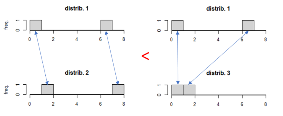

![](./figs/dist-em.png)

???

- Distribution discretisation by histograms
- Probability binning distance: sum bin-to-bin differences
- EMD (aka Wasserstein of order 1 metric): computes the effort/cost (=
  mass x distance) needed to transport the mass of one distribution to
  obtain de other.

---
class:

### CytoMDS example

.pull-left[

]

.pull-right[

- Mouse liver lymphocyte samples
- 55 samples split into 5 groups, 2 days of data acquisition (D91&
  D93)
- Earth Mover’s distances calculated with 4 channels used for
  pre-processing and QC (FSC-A, FSC-H, SSC-A, LD)

]

???

Forward scatter height (FSC-H), forward and side scatter area (FSC-A).

First observations:

- The projection highlights two major clusters of samples. One on the
  right composed most of the samples acquired on day D93 (blue
  squares). The other cluster of samples, on the left, includes mostly
  the samples from day D91 (red triangles), but also a minority of day
  D93 samples.
- Clusters cannot be attributed solely to a batch effect of
  acquisition time point.
- Percentage of variance.

---
class:

### CytoMDS example

.pull-left[

]

.pull-right[

]

???

**Shepard's diagram**, to assess how close the projected LD euclidean
distances are to their HD EMD, for each sample pair.

**Pseudo R2**: to assess to what extend the pairwise sample EMD can be
explained by the low dimensional euclidean distances on the
projection.

- The Shepard's diagram illustrates the projection quality. It shows
  that most pairwise EMD are close to the 45° identity line.
- The pseudo R2 is 0.9679, hence above the 0.95 threshold (chosen by
  default), with only two projected dimensions.

---
class:

### CytoMDS example

.pull-left[

]

.pull-right[

]

???

Correlation of characteristics of the original HD variables and LD
dimensions to help the interpretation with **bi-plots**.

- We see a strong coordination of the first coordinate, that separates
  the clusters with both the FSC-A channel median (and FSC-A standard
  deviation, not shown).
- Let looks at FSC-A.

---
class:

### CytoMDS example

---
class:

### CytoMDS example

???

- 2D plots for two representative samples, selected for their extreme
  opposite position on the first coordinate. (Using CytoPipeline)
- Comparing these two plots reveals that sample D93/A05 is a
  low-quality sample where the cell population of interest - *liver
  lymphocytes* - is extremely small, and where most events seem to
  correspond to debris or dead/dying cells, whereas sample D93/G03 is
  a good-quality sample.

### Summary

- QC, only 4 channels
- Can be applied to more, of course (see paper)
- Interpretation is important

---
class: center, middle, inverse

# Conclusions

---
class:

### Trustworthiness is key

Neighbour embedding (NE):

1. generally poor preservation of global data structures;
2. high variability in the results depending on the initialization and
   optimization scheme (UMAP vs t-SNE for example);
3. lack of interpretable tools for NE, relating LD proximities with HD
   features.

### Interpretability

- of linear approaches (PCA) is important.
- Risks of overinterpretation (rely on distances) when using
  neighourhood embeddings.
- Consider DR evaluation and/or multi-scale approaches.

???

Interpretability

- of linear approaches (PCA) or additional step to support
  interpretation of the data (CytoMDS) are important.
---
class:

.pull-left[

#### Lab: Multivariate Analysis and PCA

#### Software

`fmsne`: https://lgatto.github.io/fmsne/

```r
BiocManager::install("lgatto/fmsne")
```

```python
pip install fmsne
```

`dreval`: https://csoneson.github.io/dreval/

```r
BiocManager::install("csoneson/dreval")
```

`CytoMDS`: https://uclouvain-cbio.github.io/CytoMDS/

```r
BiocManager::install("CytoMDS")
```

`MDSvis`: https://uclouvain-cbio.github.io/MDSvis/

```r
BiocManager::install("UCLouvain-CBIO/MDSvis")
```

]

.pull-right[

#### Suggested reading

- [Modern Statistics for modern
  biology](https://www.huber.embl.de/msmb/) Susan Holmes and Wolfgang
  Huber. Chapter 7. *Multivariate Analysis*. Cambridge University
  Press.
- Kobak, D., Berens, P. *The art of using t-SNE for single-cell
  transcriptomics*. Nat Commun 10, 5416
  (2019). [10.1038/s41467-019-13056-x](https://doi.org/10.1038/s41467-019-13056-x).
- Hauchamps, P. *et al.* (2025). “Visual Quality Control with CytoMDS,
  a Bioconductor Package for Low Dimensional Representation of
  Cytometry Sample Distances.” Cytometry. Part A
  [10.1002/cyto.a.24921](https://doi.org/10.1002/cyto.a.24921).

#### Acknowledgements

**Philippe Hauchamps** (DDUV/CBIO) for `CytoMDS` and slides/figures.
**Cyril de Bodt** (EPL/ICTEAM) for `fmsne` and
slides/figures. **Axelle Loriot** (DDUV/CBIO) for PCA
examples. **Charlotte Soneson** (FMI, Basel) for discussions.

]